Explore Exploit Tradeoff
A practical guide to Bayesian optimization with visuals. Learn how it balances exploration and exploitation to find global maxima in costly black-box functions using Gaussian processes and uncertainty-based utility functions.


Navigating a Wavy Landscape with Bayesian Optimization
Bayesian optimization is a powerful method for finding the maximum of an unknown, expensive‑to‑evaluate function with as few samples as possible. In this walkthrough, we will explain how it balances exploration and exploitation, show a concrete example on a challenging test function, and highlight why it is useful for real problems.
Basically, the question we are asking is how to find the minimum or maximum of an unknown, expensive-to-evaluate process, by pure experimentation, in as few steps as possible, under some sensible input-bounds.
Let us see this process in action before we dive deeper.
Notice how closely the dotted curve (prediction) and the blue region (which represents confidence) hug the blue curve quickly within only 17 iterations. We also approach the two global maximum values of 1.075.
The Hidden Function
In our video demonstration above, the user interacts with an application that hides the true form of a simple one‑dimensional function on the interval [0, 1]. Behind the scenes the function is
f(x) = sin(2πx) + 0.5 * sin(6πx)
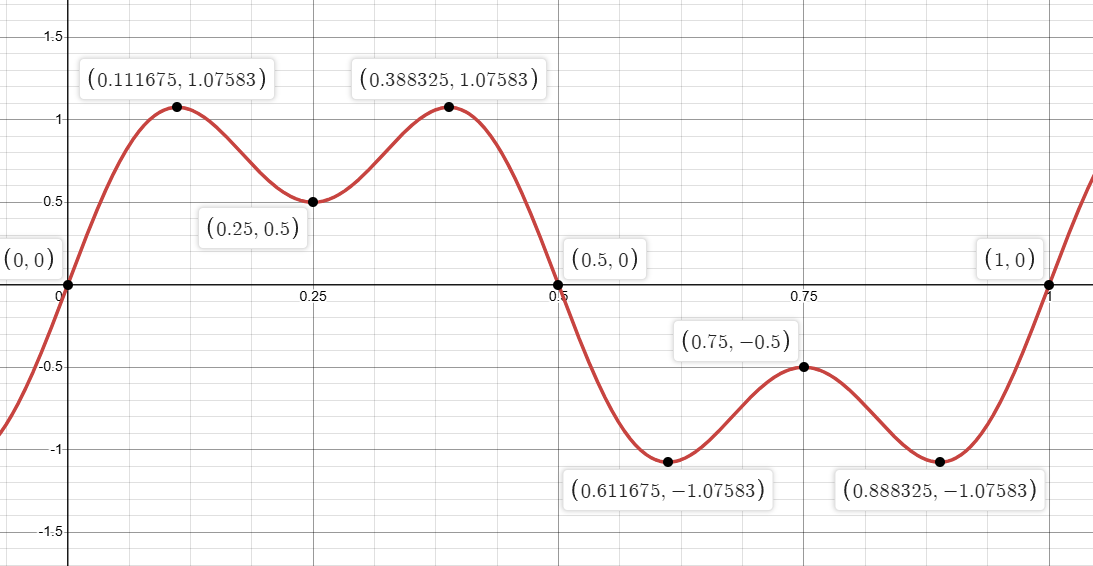
This function has six critical points:
| Type | x | f(x) |
|---|---|---|
| Local maximum | 0.25 | 0.50 |
| Local minimum | 0.75 | –0.50 |
| Global maxima | 0.11167 | 1.07583 |
| Global maxima | 0.38833 | 1.07583 |
| Global minima | 0.61167 | –1.07583 |
| Global minima | 0.88833 | –1.07583 |
The two highest peaks at x ≈ 0.1117 and x ≈ 0.3883 have the same maximum value. This wavy shape with local peaks and valleys makes it an ideal testbed to show how Bayesian optimization discovers the true maxima without being fooled by local extremes.
Real‑World Motivations
Evaluating a function can be costly in many settings. Here are three scenarios where Bayesian optimization delivers significant savings:
- Hyperparameter Tuning in Machine Learning
Training a single machine learning model can take hours or days. Grid search or random search over learning rates, regularization strengths, or network architectures may require hundreds of full training runs. Bayesian optimization finds near‑optimal settings with only a few experiments. - Materials and Chemistry Experiments
Each laboratory experiment to create a new compound or test a fabrication process can cost thousands of dollars. By treating yield, strength, or efficiency as the output of a black‑box function, Bayesian optimization can focus on the most promising candidates and avoid costly wasted trials. - A/B Testing for Web Interfaces
Running live A/B tests reduces user traffic to the current best design. By modeling metrics such as click‑through rate or conversion as a continuous function of design parameters, Bayesian optimization directs tests to the most informative variants and minimizes lost revenue.
In all these cases, each function evaluation has a real cost. Reducing the number of evaluations while still finding the global maximum is the key benefit of Bayesian optimization.
The Optimization Process
At its heart, Bayesian optimization maintains a probabilistic model i.e. typically a Gaussian process, over the unknown function. After each evaluation, the model updates its predictive mean μ(x) and standard deviation σ(x). It then uses an acquisition function U(x) to score every candidate x and select where to sample next.
Bayesian optimization works in an iterative loop:
- Model the Function with a Gaussian Process
After each evaluation, the algorithm fits a Gaussian process (GP) to the observed data. The GP provides a predictive mean μ(x) and predictive standard deviation σ(x) at every point x in [0, 1]. - Define an Acquisition Function
The acquisition function U(x) uses μ(x) and σ(x) to score every candidate x by balancing exploitation of high mean values with exploration of high‑uncertainty regions. - Select the Next Sample
The next x is chosen by maximizing U(x). The chosen point is then evaluated on the true function. - Update the Model and Repeat
The new data point is added to the GP, which updates μ(x) and σ(x). This process continues until a budget of evaluations is exhausted or the maximum is found with sufficient confidence.
A common acquisition function is the Upper Confidence Bound (UCB):
U(x) = μ(x) + κ * σ(x)
where κ controls how much the algorithm values exploration (large κ) versus exploitation (small κ). The parameter κ > 0 controls the balance between exploration and exploitation. A large κ places greater weight on σ(x), encouraging sampling in high‑uncertainty regions. Over successive steps, as uncertainty falls around sampled points, the mean term μ(x) guides the search toward the global maximum.
Other popular choices are Expected Improvement (EI) and Probability of Improvement (POI), which focus on the expected gain over the best observed value or the probability of beating it, respectively.
- Expected Improvement (EI): the expected gain over the current best known value f(x*)
Uei(x) = E[max(0, f(x) − f(x∗))]
- Probability of Improvement (POI):
Upoi(x) = Pr(f(x) > f(x∗))
Visualizing the Journey
Below we describe how the model’s predictions, uncertainty, and suggested sampling points evolve over time.
After 4 Steps
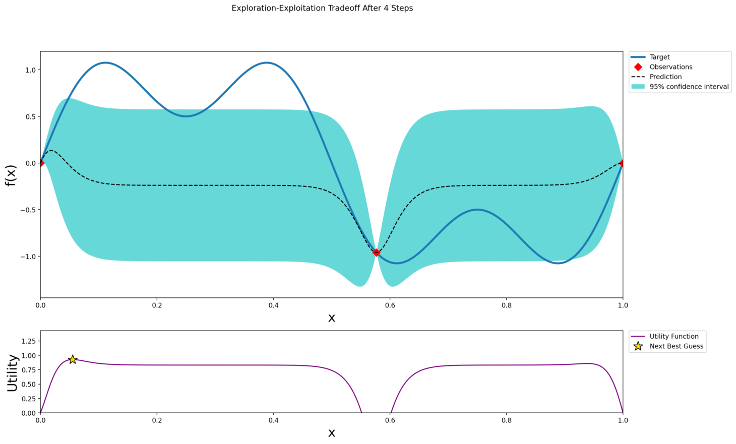
At this early stage the Gaussian process has only seen a couple of points. The predictive mean is almost flat and does not capture the wavy pattern yet. The 95 percent confidence band covers most of the interval. The acquisition function peaks where σ(x) is highest, leading the algorithm to explore where it knows the least.
After 12 Steps
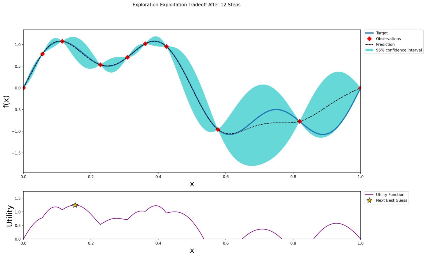
With more samples the predictive mean begins to trace the peaks and valleys of the true function. The confidence band narrows around observed points. The acquisition function now balances exploring uncertain regions and exploiting areas with higher predicted values. Notice how it avoids sampling in deep troughs that offer little chance of improvement.
After 17 Steps
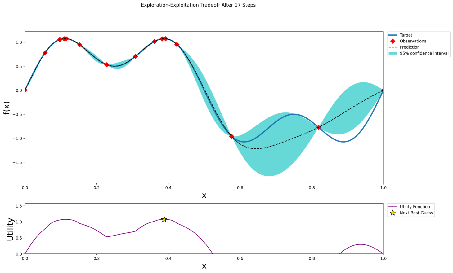
By this point the optimizer has likely discovered the two global peaks near x ≈ 0.1117 and x ≈ 0.3883. The predictive mean aligns closely with the true function around these maxima and the confidence band is tight. The acquisition function focuses on fine‑tuning between these peaks to determine which is truly highest. This process shows that Bayesian optimization efficiently avoids local maxima and converges on the global optimum.
Why Bayesian Optimization Works
Bayesian optimization delivers three main advantages:
- Sample Efficiency
It uses information from past evaluations to choose future samples that are most informative or promising. This reduces the total number of expensive evaluations. - Principled Exploration‑Exploitation Trade‑off
By quantifying uncertainty with σ(x), it naturally decides when to explore unknown regions and when to exploit high‑reward areas. - Uncertainty Quantification
The confidence intervals provided by the Gaussian process help users understand how reliably the optimizer has found the maximum.
Limitations to Consider
No optimization method is perfect. Key challenges include:
- Scalability
Gaussian process updates become computationally expensive as the number of samples grows or in higher dimensions. - Model Assumptions
The GP prior assumes a certain smoothness that may not hold for highly irregular or discontinuous functions. - Acquisition‑Function Tuning
Parameters such as κ in UCB or thresholds in EI must be chosen thoughtfully. Poor choices can lead to excessive exploration or premature exploitation. - Computational Overhead
Fitting a GP and evaluating the acquisition function on a fine grid at each iteration can limit real‑time applications.
When each function evaluation carries a real cost in time, money, or resources, Bayesian optimization provides a systematic, efficient path to the global maximum. In our wavy test function with multiple local extrema, the method reliably finds both global maxima in just a handful of samples. This approach has proven valuable for tasks ranging from hyperparameter tuning and materials discovery to A/B testing and beyond. By quantifying uncertainty and guiding sampling intelligently, Bayesian optimization offers a powerful tool for solving black‑box optimization problems.
If you're working on complex decision problems where brute-force solutions are too costly or inefficient, our team specializes in building custom machine learning and optimization pipelines tailored to your use case. Whether it's intelligent experimentation, adaptive modeling, or scalable AI workflows, we help businesses move from guesswork to smart, data-driven action.
Contact DialectAI to explore how we can bring this kind of precision to your challenges.