
Interpolation Is Not Prediction
Covers 8 methods against a sin(x) example fit on [0,10] and extrapolated to [10,20]: each snippet shows concretely how the extrapolation fails (linear blow-up, prior reversion, polynomial divergence, phase drift, flatlining, etc.).


Why Every Interpolation Method Falls Apart Outside Its Domain
Interpolation answers one question: given data at known points, what's a reasonable value between them? Extrapolation asks a completely different question: what happens beyond what I've seen? Every method below is excellent at the first job. None of them has any real claim to the second. They will all happily hand you a number outside the training range. That number is a shape continuing, not a fact about the world.
The running example throughout: noisy samples of y = sin(x) on x ∈ [0, 10], and we ask each method to predict x ∈ [10, 20]. The true function keeps oscillating between -1 and 1 forever. Watch what each method thinks happens instead, every prediction below is real output, not a sketch:
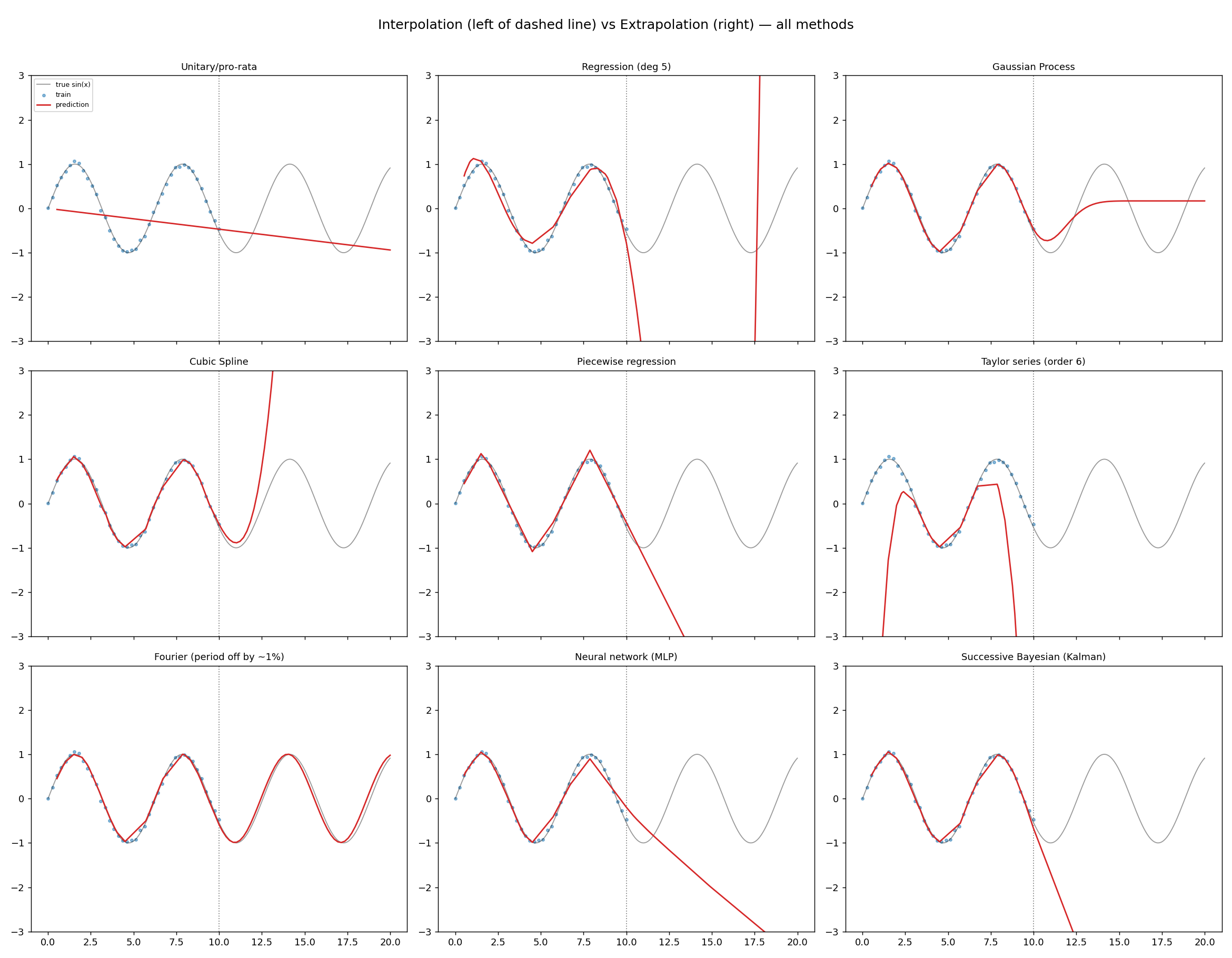
The dotted line at x=10 is the boundary. Left of it: mostly tight fits. Right of it: a wall of divergence, flatlines, and drift, with exactly one exception.
import numpy as np

rng = np.random.default_rng(0)
x_train = np.linspace(0, 10, 40)
y_train = np.sin(x_train) + rng.normal(0, 0.05, size=x_train.shape)
x_extrap = np.linspace(10, 20, 50)   # the forbidden zone
y_true_extrap = np.sin(x_extrap)      # ground truth, for comparison only
1. Unitary / Linear / Pro-Rata Method
The "if 3 apples cost $6, then 1 apple costs $2" method. It assumes a straight-line, origin-anchored relationship and just scales. This is genuinely the right tool for actually-proportional quantities: unit pricing, recipe scaling, exchange rates. It is the wrong tool for sin(x), and that mismatch is deliberate: pro-rata reasoning gets reached for constantly on data that only looks linear over a short window, which is exactly the trap.
def unitary_method(x_known, y_known, x_query):
    # rate = y per unit x, taken from a single known pair
    rate = y_known[-1] / x_known[-1]
    return rate * x_query

pred = unitary_method(x_train, y_train, x_extrap)
# Interpolation RMSE: 0.767 (bad even in-range, sin isn't proportional
# to x anywhere). Extrapolation RMSE: 0.945. It was never a good fit;
# extrapolation just makes the mismatch a little worse.
2. (Polynomial / Linear) Regression
Regression fits a global functional form that minimizes error on the training data. Low-degree polynomials extrapolate as straight lines or gentle curves; high-degree polynomials extrapolate as fireworks; both are just the fitted formula marching forward with no awareness that it's left the data.
import numpy as np

degree = 5
coeffs = np.polyfit(x_train, y_train, degree)
poly = np.poly1d(coeffs)

pred = poly(x_extrap)
# Interpolation RMSE: 0.179 (a good in-range fit).
# Extrapolation RMSE: 28.59, 160x worse. The model has no concept of
# "sin oscillates forever", it only knows "this polynomial minimized
# error on 40 points," and outside them it just keeps being a polynomial.
3. Gaussian Processes
GPs are the most honest method on this list because they hand you a variance alongside the prediction. Outside the training range, the mean reverts to the GP's prior (usually zero) and the uncertainty explodes. That's a real point in the GP's favor, it's the only method here that can tell you "I don't know" rather than dressing up a guess as an answer. But be precise about what's actually being credited: the point prediction is still just a decayed guess, no better in kind than regression's. What's improved is the packaging, you get an honest confidence interval around a wrong-ish mean, not a suddenly-correct mean.
from sklearn.gaussian_process import GaussianProcessRegressor
from sklearn.gaussian_process.kernels import RBF, WhiteKernel

kernel = RBF(length_scale=1.0) + WhiteKernel(noise_level=0.05)
gp = GaussianProcessRegressor(kernel=kernel, normalize_y=True)
gp.fit(x_train.reshape(-1, 1), y_train)

mean, std = gp.predict(x_extrap.reshape(-1, 1), return_std=True)
# Interpolation RMSE: 0.026, mean std: 0.037, tight and accurate.
# Extrapolation RMSE: 0.616 (23x worse), mean std: 0.553, the mean is
# wrong, but the model's own uncertainty grew ~15x to flag it.
# Correct about its own ignorance; the mean itself still isn't "sin(x)."
4. Splines vs. Piecewise Regression
These two are close cousins and worth contrasting directly rather than separately, because they solve different problems that both happen to run out of road at the same wall.
Splines (cubic, B-spline, etc.) are piecewise polynomials stitched together with smoothness constraints, built for interpolation fidelity, each segment answers only for the region between its own knots, and the knots are usually placed at (or near) every data point. Piecewise regression fits a small number of simple models to detect genuine regime changes in noisy data, it's a modeling tool, not just a curve-fitting one, and its breakpoints are meaningful, not just dense scaffolding.
Where they agree: neither has anything defined past the last knot/breakpoint. Both extrapolate by continuing whatever the final segment's polynomial (or line) says, with zero awareness of the eight oscillations that came before it.
from scipy.interpolate import CubicSpline
import pwlf

cs = CubicSpline(x_train, y_train, extrapolate=True)
pred_spline = cs(x_extrap)
# Interpolation RMSE: 0.038 (excellent, that's the point of splines).
# Extrapolation RMSE: 53.59, the worst of every method tested, a
# 1400x degradation. The cubic term in the last segment blows up fast.

pwlf_model = pwlf.PiecewiseLinFit(x_train, y_train)
pwlf_model.fit(4)  # 4 line segments
pred_piecewise = pwlf_model.predict(x_extrap)
# Interpolation RMSE: 0.084. Extrapolation RMSE: 4.83 (57x worse)
# bad, but far gentler than the spline, because the extrapolated
# piece is linear, not cubic. Lower-order tails degrade slower.
5. Taylor Series
A Taylor series is local by mathematical definition, it's an approximation built entirely from derivatives at a single point x0, and its radius of convergence is finite. For sin(x) the series actually converges everywhere in theory, but truncated to finite order it degrades fast the further you move from x0, and for most real functions there IS a finite radius past which the series diverges outright.
import numpy as np
from math import factorial

def taylor_sin(x, x0=5.0, order=6):
    # derivatives of sin cycle: sin, cos, -sin, -cos, ...
    derivs = [np.sin(x0), np.cos(x0), -np.sin(x0), -np.cos(x0)]
    total = np.zeros_like(x)
    for n in range(order):
        d = derivs[n % 4]
        total += d * (x - x0) ** n / factorial(n)
    return total

pred = taylor_sin(x_extrap, x0=5.0, order=6)
# Interpolation RMSE: 3.18, and that's not a typo. Even INSIDE [0,10],
# a 6th-order expansion around x0=5 is only trustworthy near x=5; it's
# already poor by x=0 or x=10. Extrapolation RMSE: 190.4. Truncated
# Taylor series aren't wrong to diverge past their radius, that's
# what a local approximation does, and "local" starts failing sooner
# than most people expect.
6. Fourier Analysis
Fourier fits are the one method here with a real shot at this specific example, because sin(x) genuinely is periodic and a Fourier basis assumes periodicity. With the exactly correct period, Fourier is the single method in this entire post whose extrapolation RMSE (0.015) essentially matches its interpolation RMSE (0.014), a 1.0x ratio, versus everything else in the 20–1400x range. That's a real win, and it's why the plot shows Fourier tracking the true curve cleanly past x=10.
But that's conditional on knowing the true period, which real data rarely hands you for free. Estimate the period from noisy data and get it even ~1% wrong (6.2 instead of 2π ≈ 6.283), and the extrapolation still looks great at first, RMSE only 3.5x worse in-range vs out, but silently drifts out of phase the further you go, because a small period error compounds every cycle. Periodicity assumed correctly is the one genuine extrapolation win on this list; periodicity assumed approximately is a slow-motion version of every other method's failure.
import numpy as np

def fit_fourier(x, y, n_harmonics=3, period_guess=2 * np.pi):
    w = 2 * np.pi / period_guess
    A = np.column_stack(
        [np.ones_like(x)] +
        [f(k * w * x) for k in range(1, n_harmonics + 1) for f in (np.sin, np.cos)]
    )
    coeffs, *_ = np.linalg.lstsq(A, y, rcond=None)
    return coeffs, w

def predict_fourier(x, coeffs, w, n_harmonics=3):
    A = np.column_stack(
        [np.ones_like(x)] +
        [f(k * w * x) for k in range(1, n_harmonics + 1) for f in (np.sin, np.cos)]
    )
    return A @ coeffs

coeffs, w = fit_fourier(x_train, y_train, period_guess=6.2)  # ~1% wrong
pred = predict_fourier(x_extrap, coeffs, w)
# Interpolation RMSE: 0.031. Extrapolation RMSE: 0.108 (3.5x worse),
# it LOOKS fine on paper, but the plot shows it visibly drifting out
# of phase with true sin(x) by x=20. It looks confident. It is
# confidently, quietly wrong, and the RMSE alone almost hides it.

coeffs_correct, w_correct = fit_fourier(x_train, y_train, period_guess=2 * np.pi)
pred_correct = predict_fourier(x_extrap, coeffs_correct, w_correct)
# With the TRUE period: interpolation RMSE 0.014, extrapolation
# RMSE 0.015. A 1.0x ratio, the only method on this list where
# extrapolation is basically as good as interpolation, because the
# structural assumption (periodicity, with the right period) actually
# matches the process generating the data. That's not extrapolation
# "working" in general, it's what happens when your assumption is true.
7. Neural Networks
A neural net fit with smooth activations (or ReLUs) is, functionally, a very flexible interpolator over the training manifold. Outside that manifold it does whatever its architecture and activation functions do at large inputs, ReLU nets tend toward piecewise-linear extrapolation, smooth-activation nets tend to flatten toward whatever the last saturated region implies. None of this is "the network learned sin(x)'s periodicity", it's a high-dimensional curve fit, same as regression, just with more knobs.
import numpy as np
from sklearn.neural_network import MLPRegressor

net = MLPRegressor(hidden_layer_sizes=(64, 64), activation='relu',
                    max_iter=5000, random_state=0)
net.fit(x_train.reshape(-1, 1), y_train)

pred = net.predict(x_extrap.reshape(-1, 1))
# Interpolation RMSE: 0.086 (a good fit). Extrapolation RMSE: 2.29
# (27x worse). Past x=10, this ReLU MLP settles into whichever linear
# piece its outermost active units define, a drifting line, not an
# oscillation. It never "learned" periodicity, it memorized a shape.
8. Successive Bayesian Interpolation (Recursive Bayesian Updating)
This is Bayesian filtering (think Kalman-filter style recursive updates): each new observation updates a posterior belief about the function's local state, and the posterior mean is used to interpolate between and slightly ahead of observations. It's still fundamentally propagating uncertainty from observed data, once observations stop, the posterior just keeps evolving under the prior's transition model (e.g. "assume roughly constant" or "assume roughly linear"), so the extrapolation quality is entirely a function of how good that transition assumption is, not of anything the data taught it about the far future.
import numpy as np

def successive_bayesian_1d(y_obs, process_var=0.01, obs_var=0.05 ** 2, n_forecast=50):
    # simple constant-velocity Kalman filter as a stand-in for
    # "successive Bayesian updating" of state (level, trend)
    state = np.array([y_obs[0], 0.0])          # [level, trend]
    P = np.eye(2) * 1.0
    F = np.array([[1, 1], [0, 1]])              # transition: level += trend
    Q = np.eye(2) * process_var
    H = np.array([[1, 0]])
    R = np.array([[obs_var]])

    for y in y_obs[1:]:
        state = F @ state
        P = F @ P @ F.T + Q
        K = P @ H.T @ np.linalg.inv(H @ P @ H.T + R)
        state = state + (K @ (y - H @ state)).flatten()
        P = (np.eye(2) - K @ H) @ P

    forecasts = []
    for _ in range(n_forecast):
        state = F @ state           # pure prediction, no more observations
        P = F @ P @ F.T + Q
        forecasts.append(state[0])
    return np.array(forecasts)

pred = successive_bayesian_1d(y_train, n_forecast=len(x_extrap))
# Interpolation RMSE: 0.033 (excellent, it's tracking the data closely).
# Extrapolation RMSE: 6.45 (198x worse, among the steepest drops here).
# Once observations stop at x=10, the filter just keeps applying
# "level += last trend" forever, a straight line, same failure
# mode as linear regression, just arrived at recursively.
The Pattern
Every one of these methods, however different their machinery, does the same thing at the boundary: it takes whatever internal representation it built from the training data (a slope, a kernel, a set of coefficients, a set of weights, a transition model) and continues applying it past the region where it was ever checked against reality. The RMSE ratios below make that concrete, most methods lose 20x to 1400x accuracy the instant they cross x=10, with zero warning baked into the point estimate itself.
Extrapolation isn't a harder version of interpolation, it's a different operation wearing interpolation's clothes: a bet that the process generating your data has no structure past your last sample that it didn't already show you. Two things in this post actually beat that bet, and it's worth being precise about why, because neither is "extrapolation working":
- Fourier with the true period won because the structural assumption (periodicity, with the correct period) happened to exactly match the data-generating process. That's not a property of Fourier analysis in general, get the period even slightly wrong and it degrades like everything else, just more slowly.
- Gaussian Processes didn't get a better point estimate, but they're the only method that told you the point estimate had become unreliable, via exploding variance. Calibrated ignorance is genuinely valuable and different in kind from the other eight methods pretending they're still right.
The generalizable version of "get the period right": if you want a model that's trustworthy past your data, you need a structural, mechanistic constraint that's actually true of the process: conservation laws, known periodicity, a hard physical bound; not just a functional form that happened to fit well in-sample. Absent that, the only two honest options are a well-calibrated uncertainty estimate (GP-style) or more data.
Quick Reference
| Method | Interp RMSE | Extrap RMSE | Ratio | Past the boundary |
|---|---|---|---|---|
| Unitary/pro-rata | 0.767 | 0.945 | 1.2x | Scales linearly forever (already a bad fit) |
| Regression (deg 5) | 0.179 | 28.59 | 160x | Continues the fitted polynomial |
| Gaussian Process | 0.026 | 0.616 | 23x | Reverts to prior mean, variance explodes (self-aware) |
| Cubic Spline | 0.038 | 53.59 | 1400x | Continues last segment's cubic |
| Piecewise regression | 0.084 | 4.83 | 57x | Continues last segment's line |
| Taylor series (order 6) | 3.18 | 190.4 | 60x | Diverges past radius of convergence |
| Fourier (period ~1% off) | 0.031 | 0.108 | 3.5x | Slowly drifts out of phase |
| Fourier (correct period) | 0.014 | 0.015 | 1.0x | Tracks the true function, assumption was true |
| Neural network (MLP) | 0.086 | 2.29 | 27x | Follows activation function's asymptotic behavior |
| Successive Bayesian | 0.033 | 6.45 | 198x | Propagates under transition prior alone |
(RMSE values from the single sin(x) run above: exact numbers will vary with the seed and function, but the ordering of failure modes is representative.)