From Derivatives to Adam: Building Optimization Intuition with PyTorch
From first and second derivatives to Adam optimizer: a hands-on walkthrough of key optimization ideas using PyTorch. Simple, minimal examples with gradients, momentum, and adaptive learning strategies to build deep intuition.


Optimization is the backbone of machine learning, statistics, and applied mathematics. In this guide, we'll walk from first principles like the first and second derivative, through classical optimizers like Gradient Descent and Momentum, and build up to the powerful Adam optimizer. We use small, intuitive examples with PyTorch to illustrate each step.
In this article, we try to explain:
- Convexity, first and second derivative tests and
- How Newton-Raphson and Gradient Descent work
- How Momentum, Nesterov Accelerated Gradient, AdaGrad, RMSProp, and Adam evolve from earlier ideas
- PyTorch implementations for each method
- A brief mention of other optimization techniques outside the scope
Derivatives and Convexity
An optimization problem minimizes a function f : Rn → R.
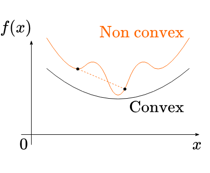
A function is convex if the line segment between any two arbitrary points on the graph lies above the graph.
A function is convex if:
f(λx + (1−λ)y ) ≤ λf(x) + (1−λ) f(y), ∀ x,y ∈ Rn, λ ∈ [0,1]
A convex function is one where the graph curves upward, like a bowl. This is important because convex functions have a nice property: any local minimum is also a global minimum, which makes them easier to work with.
What’s a Gradient? (And Why It Matters)
Imagine you're hiking on a hill, and you want to know which direction is steepest to climb or descend. The gradient of a function is like a compass pointing you in the direction of the steepest increase. In mathematical terms, the gradient is a vector of partial derivatives: it tells you how the function changes in each direction.
For example, suppose you have a simple function:
f(x,y) = x2+y2
This represents a bowl-shaped surface. The gradient is:
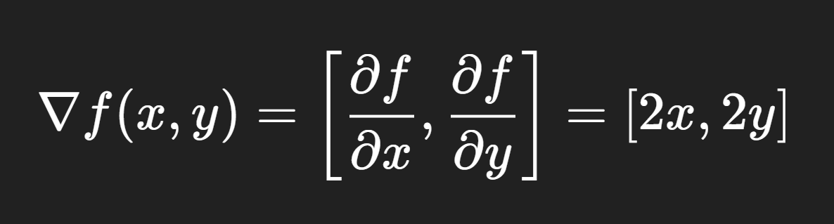
This tells you how the function increases in the x and y directions.
What’s the Hessian?
While the gradient tells you the direction of steepest ascent, the Hessian tells you how the steepness itself changes: it captures the curvature of the surface. It’s a matrix of second-order partial derivatives.
For our function:
f(x,y) = x2+y2
The Hessian is:
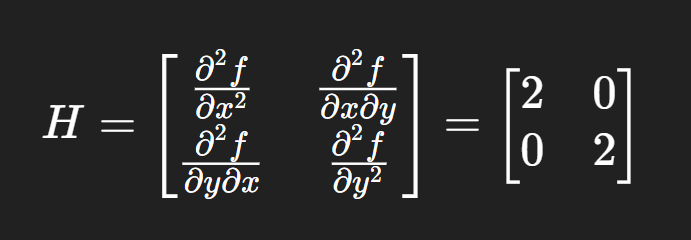
This matrix tells us how the slope (the gradient) changes as we move across the surface. Since both diagonal values are positive, the function is curving upwards in all directions.
First Derivative Test
The first derivative of a function (also called a gradient) tells us the slope or the rate of change. For scalar functions:
- Positive gradient: function is increasing
- Negative gradient: function is decreasing
A local minimum denoted by x∗ satisfies ∇f(x∗) = 0 i.e. the derivative (equivalently slope or tangent) at a minima or maxima will be zero.
Second Derivative Test
The second derivative tells us about curvature:
- Positive: convex (minimum possible)
- Negative: concave (maximum possible)
If ∇f(x∗) = 0 and ∇2f(x∗ ) ≻ 0, then x∗ is a local minimum.
What Does “Positive Semi-Definite” Mean?
A matrix is positive semi-definite if it never "curves down": meaning, the function either curves up or stays flat. In our example, the Hessian matrix has positive values on the diagonal and zero elsewhere, so it is positive definite (which is even stronger than semi-definite).
Because the Hessian above is positive semi-definite everywhere (in fact, it’s constant and always the same), we can say that: f(x,y)=x2+y2 is a convex function.
Here’s a breakdown of the different types of definiteness, how many types there are, and what they mean.
| Type | Symbolic Condition | Eigenvalues | Curvature Meaning | Function Shape |
|---|---|---|---|---|
| Positive Definite | for all | All positive | Curves upward in every direction | Bowl (strictly convex) |
| Positive Semi-Definite | for all | All non-negative | Curves upward or flat, never downward | Flat bowl or valley |
| Negative Definite | for all | All negative | Curves downward in every direction | Dome (strictly concave) |
| Negative Semi-Definite | for all | All non-positive | Curves downward or flat, never upward | Flat dome or ridge |
| Indefinite | can be positive or negative | Mixed signs | Curves up in some directions, down in others | Saddle shape |
Summary:
- Positive Definite: Think of a round bowl: every direction curves upward → convex.
- Positive Semi-Definite: Like a bowl with some flat directions → still convex, but less strict.
- Negative Definite: Upside-down bowl: curves downward → concave.
- Negative Semi-Definite: Flat dome or ridge: never curves upward.
- Indefinite: Saddle: some directions curve up, others down → not convex or concave.
Why This Matters for Optimization
- For minimization problems, we want the function to be convex.
- So, check whether the function's Hessian is positive semi-definite (or definite) in our region of interest.
- If it’s indefinite, the function has saddle points; trickier to optimize.
Here’s how to compute gradient and Hessian in PyTorch:
import torch

x = torch.tensor([2.0], requires_grad=True)
def f(x):
    return (x - 3) ** 2

# First derivative
y = f(x)
y.backward() # ∇f(x)
print('Gradient:', x.grad.item())  # Should be 2*(x - 3)

# Second derivative (Hessian for 1D)
x = torch.tensor([2.0], requires_grad=True)
y = f(x)
g = torch.autograd.grad(y, x, create_graph=True)[0] # ∇²f(x)
H = torch.autograd.grad(g, x)[0]
print('Hessian:', H.item())  # Should be 2
Remember:
- Gradient = direction of steepest change.
- Hessian = how that steepest direction changes (the curvature).
- If the Hessian is positive semi-definite everywhere, the function is convex — like a bowl that never dips down.
A quick preview of how the different optimizers behave on toy optimization problems. We are looking at each step that optimizers take to reach the minimum.
The code provided in this article to understand these optimizers is available in this Kaggle notebook.
Newton-Raphson Method for Minimization
Originally used to find roots f(x) = 0, we adapt Newton-Raphson to find stationary points ∇f(x) = 0:
xk+1 = xk − (∇ f(xk) / [∇2 f(xk)] )
Explanation:
- ∇f(xk): gradient (slope)
- ∇2f(xk): Hessian (curvature)
- This step updates xk by moving in the direction of zero slope, adjusted by curvature
This is slightly different from the original Newton Raphson method since we are moving in the direction of the slope tending to zero (finding gradient's root) instead of the value of the function (finding function's root), notice how the fraction is gradient-over-hessian instead of the function-over-gradient.
The convergence to minimum is quite fast, even if the initialization is very far and requires very few steps to find the minimum.
PyTorch snippet (for 1D):
# The value of x also represents our initial guess or starting position
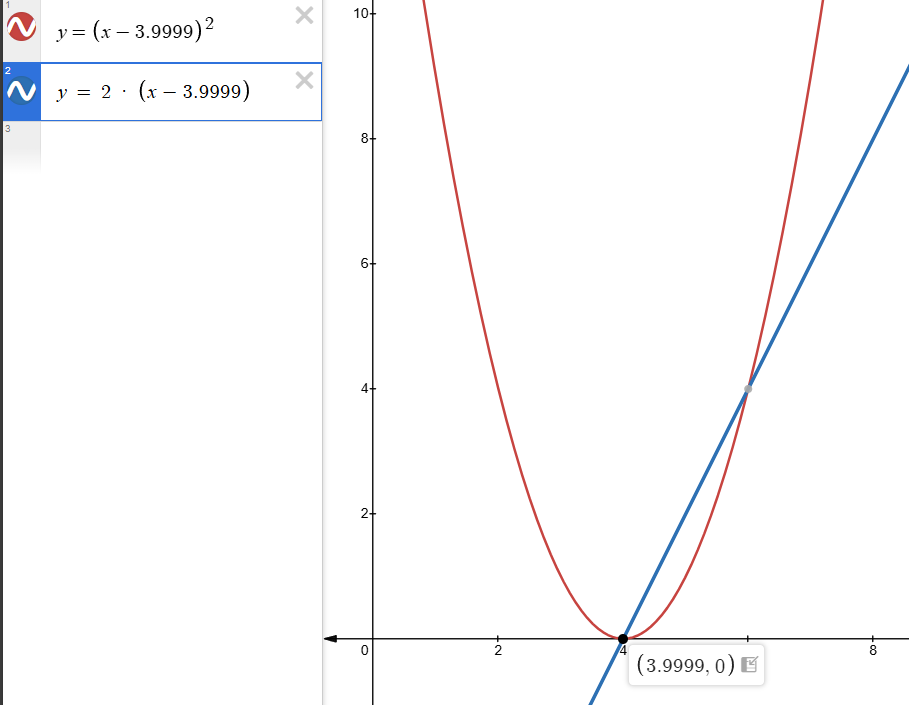
x = torch.tensor([9999.0], requires_grad=True)
for _ in range(5):
f = (x - 3.9999)**2
grad = torch.autograd.grad(f, x, create_graph=True)[0]
hess = torch.autograd.grad(grad, x, create_graph=True)[0]
with torch.no_grad():
x -= grad / hess
print(x.item())
print("Newton result:", x.item()) # The answer should be very close to 3.9999
Limitations:
- Requires second derivative (expensive in high-dimensions)
- Not stable unless function is very smooth
Gradient Descent (GD)
Gradient Descent updates the variable in the direction opposite to the gradient of the loss function.
The update rule is:
xk+1 = xk − η∇f(xk)
Terms:
- xk: current value of the parameter
- η: learning rate (step size), a small positive scalar
- ∇f(xk): gradient (direction of steepest ascent) of the function at xk
No second derivative is involved, we move in the direction of negative gradient to reach the minimum. Convergence to minima is dependent on initialization and learning rate. If initialization is far from minima it will require more steps (requires tuning learning rate) and might stop early.
PyTorch version:
import torch

x = torch.tensor([2.0], requires_grad=True) #initialization
lr = 0.1 # learning rate

for i in range(20):
    f = (x - 3)**2
    f.backward()
    with torch.no_grad():
        x -= lr * x.grad
    x = x.grad.zero_()
    print(f"Result at step {i+1} : {x.item()}")


print("GD result:", x.item())
Try increasing the value of x to a very large number in the above code snippet to notice that it takes more steps (20) to converge and needs lr to be tuned for convergence to be achieved.
Stochastic Gradient Descent (SGD)
SGD follows the same update rule as Gradient Descent, but instead of using the full dataset (or exact function), it uses a randomly selected subset (mini-batch). It introduces noise but often improves generalization.
Use PyTorch’s built-in SGD:
import torch

x = torch.nn.Parameter(torch.tensor([2.0]))
opt = torch.optim.SGD([x], lr=0.1) # omitted momentum argument (next method)

for i in range(20):
    loss = (x - 3)**2
    opt.zero_grad()
    loss.backward()
    opt.step()
    print(f"Result at step {i+1} : {x.item()}")


print("SGD result:", x.item())
Momentum
Momentum adds a velocity term that accumulates gradients over time, allowing the optimizer to gain speed in directions with consistent gradient:
vk+1 = β vk + η∇ f(xk)
xk+1 = xk − vk+1
Terms:
- vk: velocity (running average of gradients)
- β: momentum coefficient (e.g., 0.9)
- η: learning rate (step size), a small positive scalar
PyTorch implementation:
import torch

x = torch.tensor([5.0], requires_grad=True)

def f(x): return (x - 3)**2

v = torch.tensor([0.0])
lr = 0.1
beta = 0.9

for i in range(50):
    y = f(x)
    y.backward()
    with torch.no_grad():
        v = beta * v + lr * x.grad # calculating momentum
        x -= v
        _ = x.grad.zero_()
    print(f"Result at step {i+1} : {x.item()}")

print('Momentum Result:', x.item())
OR
import torch

x = torch.nn.Parameter(torch.tensor([2.0]))
opt = torch.optim.SGD([x], lr=0.1, momentum=0.9)

for i in range(20):
    loss = (x - 3)**2
    opt.zero_grad()
    loss.backward()
    opt.step()
    print(f"Result at step {i+1} : {x.item()}")

print("Momentum result:", x.item())
Nesterov Accelerated Gradient (NAG)
NAG improves upon momentum by computing the gradient after a lookahead step:
xlookahead = xk − βvk
vk+1 = βvk + η∇ f(xlookahead)
xk+1 = xk − vk+1
Terms:
- xlookahead : lookahead point
- vk+1 : updated velocity
This anticipates the next step and can lead to faster convergence.
In PyTorch:
import torch

x = torch.tensor([0.0], requires_grad=True)
def f(x): return (x - 3)**2

v = torch.tensor([0.0])
lr = 0.1
beta = 0.9

for i in range(50):
    x_lookahead = x - beta * v
    x_lookahead.retain_grad()
    y = f(x_lookahead)
    y.backward()
    with torch.no_grad():
        v = beta * v + lr * x_lookahead.grad
        x -= v
        _ = x.grad.zero_()
    print(f"Result at step {i+1} : {x.item()}")


print('NAG Result:', x.item())
OR
import torch

x = torch.nn.Parameter(torch.tensor([2.0]))
opt = torch.optim.SGD([x], lr=0.1, momentum=0.9, nesterov=True)

for i in range(20):
    loss = (x - 3)**2
    opt.zero_grad()
    loss.backward()
    opt.step()
    print(f"Result at step {i+1} : {x.item()}")

print("NAG result:", x.item())
AdaGrad
AdaGrad adapts the learning rate for each parameter by scaling inversely proportional to the square root of past squared gradients:
Gk = Gk−1 + (∇ f(xk))2
xk+1 = xk − ( η / ( sqrt(Gk) + ϵ)) ∇f(xk)
Terms:
- Gk: sum of past squared gradients (per-dimension)
- ϵ: small constant to prevent divide-by-zero
PyTorch:
import torch

x = torch.tensor([0.0], requires_grad=True)
def f(x): return (x - 3)**2

G = torch.tensor([0.0])
eps = 1e-8
lr = 0.5

for i in range(50):
    y = f(x)
    y.backward()
    with torch.no_grad():
        G += x.grad**2
        x -= lr / (G.sqrt() + eps) * x.grad
        _ = x.grad.zero_()
    print(f"Result at step {i+1} : {x.item()}")


print('AdaGrad Result:', x.item())
import torch
x = torch.nn.Parameter(torch.tensor([2.0]))
opt = torch.optim.Adagrad([x], lr=0.5)
for i in range(20):
loss = (x - 3)**2
opt.zero_grad()
loss.backward()
opt.step()
print(f"Result at step {i+1} : {x.item()}")
print("Adagrad result:", x.item())
RMSProp
RMSProp fixes AdaGrad's aggressively shrinking learning rate by using an exponentially weighted moving average of squared gradients:
Gk=β Gk−1 + (1−β)∇ f(xk)2
xk+1 = xk − ( η / ( sqrt(Gk) + ϵ)) ∇f(xk)
Terms:
- β: decay factor (e.g. 0.9)
The second equation i.e. the update rule is the same as AdaGrad.
PyTorch:
import torch

x = torch.tensor([0.0], requires_grad=True)
def f(x): return (x - 3)**2

G = torch.tensor([0.0])
gamma = 0.9
lr = 0.1
eps = 1e-8

for i in range(50):
    y = f(x)
    y.backward()
    with torch.no_grad():
        G = gamma * G + (1 - gamma) * x.grad**2
        x -= lr / (G.sqrt() + eps) * x.grad
        _ = x.grad.zero_()
    print(f"Result at step {i+1} : {x.item()}")


print('RMSProp Result:', x.item())
OR
import torch

x = torch.nn.Parameter(torch.tensor([2.0]))
opt = torch.optim.RMSprop([x], lr=0.1, alpha=0.9)

for i in range(20):
    loss = (x - 3)**2
    opt.zero_grad()
    loss.backward()
    opt.step()
    print(f"Result at step {i+1} : {x.item()}")


print("RMSProp result:", x.item())
Adam Optimizer
Adam combines Momentum + RMSProp with bias correction. Adam which stands for Adaptive Moment Estimation combines ideas from Momentum and RMSProp. It keeps track of both the mean and uncentered variance of the gradients:
mk = β1mk−1 + (1−β1) ∇f(xk) (1st moment)
vk = β2vk-1 + (1−β2) ∇f(xk)2 (2nd moment)
m'k = mk / (1−β1k)
v'k = vk / (1−β2k)
xk+1 = xk − ηm'k / (sqrt(v'k) + ϵ)
Terms:
- mk: exponential moving average of gradients (1st moment)
- vk: exponential moving average of squared gradients (2nd moment)
- β1,β2: decay rates for moment estimates (default: 0.9, 0.999)
- ϵ : small constant for numerical stability
PyTorch:
import torch

x = torch.tensor([0.0], requires_grad=True)
def f(x): return (x - 3)**2

m = torch.tensor([0.0])
v = torch.tensor([0.0])
beta1, beta2 = 0.9, 0.999
lr = 0.1
eps = 1e-8

for t in range(1, 51):
    y = f(x)
    y.backward()
    with torch.no_grad():
        g = x.grad
        m = beta1 * m + (1 - beta1) * g
        v = beta2 * v + (1 - beta2) * g**2
        m_hat = m / (1 - beta1**t)
        v_hat = v / (1 - beta2**t)
        x -= lr * m_hat / (v_hat.sqrt() + eps)
        _ = x.grad.zero_()
    print(f"Result at step {t} : {x.item()}")


print('Adam Result:', x.item())
OR
import torch

x = torch.nn.Parameter(torch.tensor([2.0]))
opt = torch.optim.Adam([x], lr=0.1)

for i in range(20):
    loss = (x - 3)**2
    opt.zero_grad()
    loss.backward()
    opt.step()
    print(f"Result at step {i+1} : {x.item()}")

print("Adam result:", x.item())
What We Didn’t Cover:
Second-Order and Constrained Optimization
There exist powerful methods in libraries and tools like SciPy, COIN-OR, IPOPT, cvxpy, Gurobi, etc., that go beyond first-order optimizers:
- Interior-Point Methods
- Trust-Region Methods
- Sequential Least Squares Programming (SLSQP)
- Newton-CG, BFGS, L-BFGS
These are useful when:
- You need exact Hessians (second derivatives)
- You have complex equality/inequality constraints
- The problem is small enough for expensive matrix operations
But these optimizers are not amenable to deep learning since
- These aren’t easily scalable to high dimensions or GPU workloads.
- PyTorch is mostly used for first-order optimizers in deep learning.
- These are best used via SciPy's scipy.optimize.minimize() and other minimization packages and tools like cvxpy, IPOPT etc., although GPU support and related speedup is limited.
Hence these methods are especially useful for small-to-medium-sized constrained optimization problems, or when second-order information (like Hessians) is cheap to compute.
We explored optimization from first principles through a progression of ideas, each adding something new:
- Gradient Descent: basic local slope
- Momentum/Nesterov: smoothing with inertia
- AdaGrad/RMSProp: adaptive step sizes
- Adam: combines momentum and RMSProp with bias correction
Understanding each helps demystify why Adam became the go-to optimizer for deep learning.